从头开始构建和训练 Transformer（上）

1、导读

2017 年，Google 研究团队发表了一篇名为《Attention Is All You Need》的论文，提出了 Transformer 架构，是机器学习，特别是深度学习和自然语言处理领域的范式转变。

Transformer 具有并行处理功能，可以实现更高效、可扩展的模型，从而更容易在大型数据集上训练它们。它还在情感分析和文本生成任务等多项 NLP 任务中表现出了卓越的性能。

在本笔记本中，我们将探索 Transformer 架构及其所有组件。我将使用 PyTorch 构建所有必要的结构和块，并且我将在 PyTorch 上使用从头开始编Transformer。

python"># 导入库

# PyTorch 
import torch 
import torch.nn as nn 
from torch.utils.data import Dataset, DataLoader, random_split 
from torch.utils.tensorboard import SummaryWriter 

# Math 
import math 

# HuggingFace 库
from datasets import load_dataset 
from tokenizers import Tokenizer 
from tokenizers .models import WordLevel 
from tokenizers.trainers import WordLevelTrainer 
from tokenizers.pre_tokenizers import Whitespace 

# Pathlib 
from pathlib import Path 

# Typing 
from Typing import  Any 

# 循环中进度条的库
from tqdm import tqdm 

# 导入警告库
import warnings

2、Transformer 架构

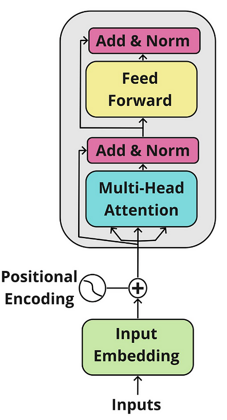
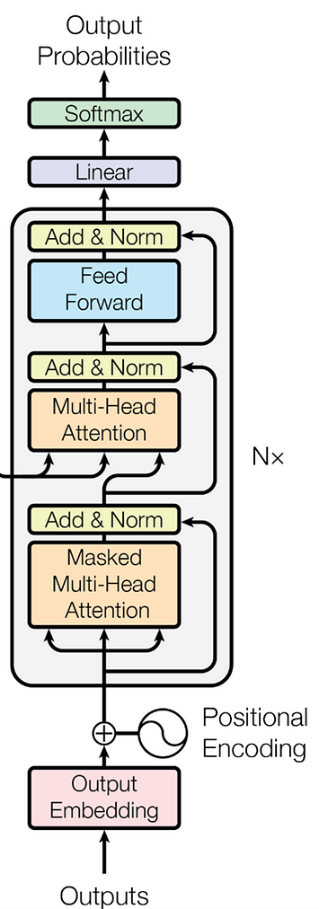
在编码之前，我们先看一下Transformer的架构。

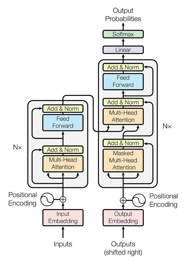
Transformer 架构有两个主要模块：编码器和解码器。让我们进一步看看它们。

编码器：它具有多头注意力机制和全连接的前馈网络。两个子层周围还有残差连接，以及每个子层输出的层归一化。模型中的所有子层和嵌入层都会产生维度 𝑑_𝑚𝑜𝑑𝑒𝑙=512 的输出。

解码器：解码器遵循类似的结构，但它插入了第三个子层，该子层对编码器块的输出执行多头关注。解码器块中的自注意子层也进行了修改，以避免位置关注后续位置。这种掩蔽确保位置 𝑖 的预测仅取决于小于𝑖 的位置处的已知输出。

编码器和解码块都重复 𝑁 次。在原始论文中，他们定义了𝑁 = 6，我们将在本笔记本中定义类似的值。

3、输入嵌入

当我们观察上面的 Transformer 架构图像时，我们可以看到嵌入代表了两个块的第一步。

下面的类InputEmbedding负责将输入文本转换为d_model维度的数值向量。为了防止我们的输入嵌入变得非常小，我们通过将它们乘以 √𝑑_𝑚𝑜𝑑𝑒𝑙 来对其进行标准化。

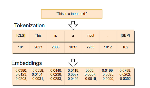
在下图中，我们可以看到嵌入是如何创建的。首先，我们有一个被分成标记的句子——我们稍后将探讨标记是什么——。然后，令牌 ID（识别号）被转换为嵌入，即高维向量。

python">class InputEmbeddings(nn.Module):
    
    def __init__(self, d_model: int, vocab_size: int):
        super().__init__()
        self.d_model = d_model # Dimension of vectors (512)
        self.vocab_size = vocab_size # Size of the vocabulary
        self.embedding = nn.Embedding(vocab_size, d_model) # PyTorch layer that converts integer indices to dense embeddings
        
    def forward(self, x):
        return self.embedding(x) * math.sqrt(self.d_model) # Normalizing the variance of the embeddings

4、位置编码

在原始论文中，作者将位置编码添加到编码器和解码器块底部的输入嵌入中，以便模型可以获得有关序列中标记的相对或绝对位置的一些信息。位置编码与嵌入具有相同的维度𝑑_模型，因此可以将两个向量相加，并且我们可以将来自单词嵌入的语义内容和来自位置编码的位置信息结合起来。

下面我们将创建一个尺寸为的PositionalEncoding位置编码矩阵。我们首先用0填充它。然后，我们将正弦函数应用于位置编码矩阵的偶数索引，而余弦函数应用于奇数索引。pe(seq_len, d_model)

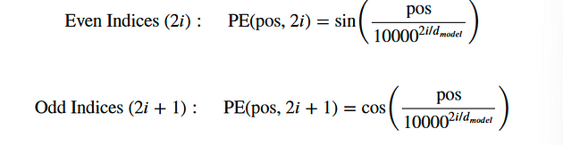
我们应用正弦和余弦函数，因为它允许模型根据序列中其他单词的位置来确定单词的位置，因为对于任何固定偏移量𝑃𝐸ₚₒₛ ₊ ₖ可以表示为𝑃𝐸ₚₒₛ 的线性函数。发生这种情况是由于正弦和余弦函数的特性，其中输入的变化会导致输出发生可预测的变化。

python">class PositionalEncoding(nn.Module):
    
    def __init__(self, d_model: int, seq_len: int, dropout: float) -> None:
        super().__init__()
        self.d_model = d_model # Dimensionality of the model
        self.seq_len = seq_len # Maximum sequence length
        self.dropout = nn.Dropout(dropout) # Dropout layer to prevent overfitting
        
        # Creating a positional encoding matrix of shape (seq_len, d_model) filled with zeros
        pe = torch.zeros(seq_len, d_model) 
        
        # Creating a tensor representing positions (0 to seq_len - 1)
        position = torch.arange(0, seq_len, dtype = torch.float).unsqueeze(1) # Transforming 'position' into a 2D tensor['seq_len, 1']
        
        # Creating the division term for the positional encoding formula
        div_term = torch.exp(torch.arange(0, d_model, 2).float() * (-math.log(10000.0) / d_model))
        
        # Apply sine to even indices in pe
        pe[:, 0::2] = torch.sin(position * div_term)
        # Apply cosine to odd indices in pe
        pe[:, 1::2] = torch.cos(position * div_term)
        
        # Adding an extra dimension at the beginning of pe matrix for batch handling
        pe = pe.unsqueeze(0)
        
        # Registering 'pe' as buffer. Buffer is a tensor not considered as a model parameter
        self.register_buffer('pe', pe) 
        
    def forward(self,x):
        # Addind positional encoding to the input tensor X
        x = x + (self.pe[:, :x.shape[1], :]).requires_grad_(False)
        return self.dropout(x) # Dropout for regularization

5、层归一化

当我们查看编码器和解码器块时，我们会看到几个称为Add & Norm的归一化层。

下面的类LayerNormalization对输入数据执行层归一化。在前向传播过程中，我们计算输入数据的平均值和标准差。然后，我们通过减去平均值并除以标准差加上一个称为epsilon的小数来标准化输入数据，以避免被零除。此过程会产生平均值为 0、标准差为 1 的标准化输出。

然后，我们将通过可学习参数缩放标准化输出alpha，并添加一个名为的可学习参数bias。训练过程负责调整这些参数。最终结果是层归一化张量，它确保网络中各层的输入规模一致。

python"># Creating Layer Normalization
class LayerNormalization(nn.Module):
    
    def __init__(self, eps: float = 10**-6) -> None: # We define epsilon as 0.000001 to avoid division by zero
        super().__init__()
        self.eps = eps
        
        # We define alpha as a trainable parameter and initialize it with ones
        self.alpha = nn.Parameter(torch.ones(1)) # One-dimensional tensor that will be used to scale the input data
        
        # We define bias as a trainable parameter and initialize it with zeros
        self.bias = nn.Parameter(torch.zeros(1)) # One-dimensional tenso that will be added to the input data
        
    def forward(self, x):
        mean = x.mean(dim = -1, keepdim = True) # Computing the mean of the input data. Keeping the number of dimensions unchanged
        std = x.std(dim = -1, keepdim = True) # Computing the standard deviation of the input data. Keeping the number of dimensions unchanged
        
        # Returning the normalized input
        return self.alpha * (x-mean) / (std + self.eps) + self.bias

6、前馈网络

在全连接前馈网络中，我们应用两个线性变换，并在其间使用 ReLU 激活。我们可以用数学方式将该操作表示为：

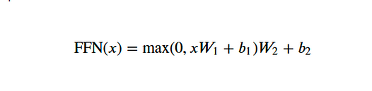
W1 和W2 是权重，而b1 和b2 是两个线性变换的偏差。

下面FeedForwardBlock，我们将定义两个线性变换 -self.linear_1和self.linear_2- 以及内层d_ff。输入数据将首先经过self.linear_1转换，将其维度从d_model增加到d_ff。

此操作的输出通过 ReLU 激活函数，该函数引入了非线性，因此网络可以学习更复杂的模式，并且该self.dropout层用于减轻过度拟合。最后的操作是self.linear_2转换为 dropout-modified 张量，将其转换回原始d_model维度。

python"># 创建前馈层
class FeedForwardBlock(nn.Module):
    
    def __init__(self, d_model: int, d_ff: int, dropout: float) -> None:
        super().__init__()
          # 第一次线性变换
        self.linear_1 = nn.Linear(d_model, d_ff) # W1 & b1
        self.dropout = nn.Dropout(dropout) # Dropout to prevent overfitting
          # 第二次线性变换
        self.linear_2 = nn.Linear(d_ff, d_model) # W2 & b2
        
    def forward(self, x):
        # (Batch, seq_len, d_model) --> (batch, seq_len, d_ff) -->(batch, seq_len, d_model)
        return self.linear_2(self.dropout(torch.relu(self.linear_1(x))))

7、多头注意力

多头注意力是 Transformer 最关键的组成部分。它负责帮助模型理解数据中的复杂关系和模式。

下图显示了多头注意力机制的工作原理。它不包括batch维度，因为它仅说明一个句子的过程。

多头注意力模块接收分为查询、键和值的输入数据，并组织成矩阵𝑄、𝐾和𝑉。每个矩阵包含输入的不同方面，并且它们具有与输入相同的维度。

然后，我们通过各自的权重矩阵𝑊^Q、𝑊^K和𝑊^V来对每个矩阵进行线性变换。这些转换将产生新的矩阵𝑄′、𝐾′和𝑉′，它们将被分成与不同头ℎ相对应的更小的矩阵，从而允许模型并行处理来自不同表示子空间的信息。这种分割为每个头创建多组查询、键和值。

最后，我们将每个头连接成一个𝐻矩阵，然后由另一个权重矩阵𝑊𝑜进行转换以产生多头注意力输出，即保留输入维度的矩阵𝑀𝐻−𝐴 。

python"># 创建多头注意力区块
class MultiHeadAttentionBlock(nn.Module):
    
    def __init__(self, d_model: int, h: int, dropout: float) -> None: # h = number of heads
        super().__init__()
        self.d_model = d_model
        self.h = h
        
        # 我们确保模型的维度可以被头的数量整除
        assert d_model % h == 0, 'd_model is not divisible by h'
        
        # d_k 是每个注意力的维度head 的键、查询和值向量
        self.d_k = d_model // h # d_k 公式，就像原始的“Attention Is All You Need”论文中一样
        
        # 定义权重矩阵
        self.w_q = nn.Linear(d_model, d_model) # W_q
        self.w_k = nn.Linear(d_model, d_model) # W_k
        self.w_v = nn.Linear(d_model, d_model) # W_v
        self.w_o = nn.Linear(d_model, d_model) # W_o
        
        self.dropout = nn.Dropout(dropout) # Dropout 层以避免过度拟合
        
    
    @staticmethod
    def attention(query, key, value, mask, dropout: nn.Dropout):# mask => 当我们希望某些单词不与其他单词交互时，我们“隐藏”它们
        
        d_k = query.shape[-1] # 查询、键和值的最后一个维度
        
        # 我们按照上图中的公式计算 Attention(Q,K,V) 
        attention_scores = (query @ key.transpose(-2,-1)) / math.sqrt(d_k) # @ = Matrix multiplication sign in PyTorch
        
        # 在应用 softmax 之前，我们应用掩码来隐藏单词之间的一些交互
        if mask is not None: # 如果定义了掩码.. .
            attention_scores.masked_fill_(mask == 0, -1e9) # 将 mask 等于 0 的每个值替换为 -1e9
        attention_scores = attention_scores.softmax(dim = -1) 
        if dropout is not None: 
            attention_scores = dropout(attention_scores) # 我们使用 dropout 来防止过拟合
            
        return (attention_scores @ value), attention_scores # 将输出矩阵乘以 V 矩阵，公式如下
        
    def forward(self, q, k, v, mask):  
        query = self.w_q(q) # Q' matrix
        key = self.w_k(k) # K' matrix
        value = self.w_v(v) # V' matrix
        
        # 将结果拆分为不同头的较小矩阵
        # 将嵌入（第三维）拆分为 h 个部分
        query = query.view(query.shape[0], query.shape[1], self.h, self.d_k).transpose(1,2) # Transpose => 将头部带到第二个维度
        key = key.view(key.shape[0], key.shape[1], self.h, self.d_k).transpose(1,2) # Transpose => 将头部带到第二个维度
        value = value.view(value.shape[0], value.shape[1], self.h, self.d_k).transpose(1,2) # Transpose => 将头部带到第二个维度
        # 获取输出和注意力分数
        x, self.attention_scores = MultiHeadAttentionBlock.attention(query, key, value, mask, self.dropout)
        # 获取H矩阵
        x = x.transpose(1, 2).contiguous().view(x.shape[0], -1, self.h * self.d_k)
        return self.w_o(x) # Multiply the H matrix by the weight matrix W_o, resulting in the MH-A matrix

8、剩余连接

当我们查看 Transformer 的架构时，我们看到每个子层（包括自注意力和前馈块）在将其传递到Add & Norm层之前将其输出添加到输入。此方法将输出与Add & Norm层中的原始输入集成。这个过程称为跳跃连接，它允许 Transformer 通过为反向传播期间梯度流经提供捷径来更有效地训练深度网络。

下面的类ResidualConnection负责这个过程。

python"># 构建剩余连接
class ResidualConnection(nn.Module):
    def __init__(self, dropout: float) -> None:
        super().__init__()
        self.dropout = nn.Dropout(dropout) # 我们使用 dropout 层来防止过度拟合
        self.norm = LayerNormalization() # 我们使用归一化层
    
    def forward(self, x, sublayer):
       # 我们对输入进行归一化并将其添加到原始输入“x”。这将创建剩余连接过程。
        return x + self.dropout(sublayer(self.norm(x)))

9、编码器

我们现在将构建编码器。我们创建的EncoderBlock类由多头注意力层和前馈层以及残差连接组成。

在原始论文中，编码器块重复六次。我们将Encoder类创建为多个 s 的集合EncoderBlock。在通过其所有块处理输入之后，我们还添加层归一化作为最后一步。

python"># 构建编码器模块
class EncoderBlock(nn.Module):
    
    # 该程序块接收多头注意程序块和前馈程序块，以及剩余连接的中断率
    def __init__(self, self_attention_block: MultiHeadAttentionBlock, feed_forward_block: FeedForwardBlock, dropout: float) -> None:
        super().__init__()
        # 存储自我注意区块和前馈区块
        self.self_attention_block = self_attention_block
        self.feed_forward_block = feed_forward_block
        self.residual_connections = nn.ModuleList([ResidualConnection(dropout) for _ in range(2)]) 
        
    def forward(self, x, src_mask):
        # 将第一个残余连接应用于自我关注区块
        x = self.residual_connections[0](x, lambda x: self.self_attention_block(x, x, x, src_mask)) # 三个 "x "分别对应查询、键和值输入以及源掩码
        
        # 将第二个残差连接应用于前馈区块
        x = self.residual_connections[1](x, self.feed_forward_block)
        return x

python"># 建设编码器
# 一个编码器可以有多个编码器模块
class Encoder(nn.Module):
    
    # 编码器接收 "EncoderBlock "实例
    def __init__(self, layers: nn.ModuleList) -> None:
        super().__init__()
        self.layers = layers # 存储编码器块
        self.norm = LayerNormalization() # 编码器层输出标准化层
        
    def forward(self, x, mask):
        # 遍历存储在 self.layers 中的每个编码器块
        for layer in self.layers:
            x = layer(x, mask) # 对输入张量 "x "应用每个编码器块
        return self.norm(x)

10、解码器

类似地，Decoder 也由几个 DecoderBlock 组成，在原论文中重复了六次。主要区别在于它有一个额外的子层，该子层通过交叉注意组件执行多头注意，该交叉注意组件使用编码器的输出作为其键和值，同时使用解码器的输入作为查询。

对于输出嵌入，我们可以使用InputEmbeddings与编码器相同的类。您还可以注意到，自注意力子层被屏蔽，这限制了模型访问序列中的未来元素。

我们将从构建类开始DecoderBlock，然后构建类Decoder，它将组装多个DecoderBlocks。

python"># 构建解码器模块
class DecoderBlock(nn.Module):
    
    # 解码器模块接收两个多头注意力模块。一个是自注意，另一个是交叉注意。
    def __init__(self,  self_attention_block: MultiHeadAttentionBlock, cross_attention_block: MultiHeadAttentionBlock, feed_forward_block: FeedForwardBlock, dropout: float) -> None:
        super().__init__()
        self.self_attention_block = self_attention_block
        self.cross_attention_block = cross_attention_block
        self.feed_forward_block = feed_forward_block
        self.residual_connections = nn.ModuleList([ResidualConnection(dropout) for _ in range(3)]) 
        
    def forward(self, x, encoder_output, src_mask, tgt_mask):
        
        # 包含查询、关键字和值以及目标语言掩码的自关注块
        x = self.residual_connections[0](x, lambda x: self.self_attention_block(x, x, x, tgt_mask))
        
        # 交叉注意代码块使用两个 "encoder_ouput "来输入键和值，再加上源语言掩码。它还接收用于解码器查询的'x'。
        x = self.residual_connections[1](x, lambda x: self.cross_attention_block(x, encoder_output, encoder_output, src_mask))
        
        # 带有残余连接的前馈区块
        x = self.residual_connections[2](x, self.feed_forward_block)
        return x

python"># 构建解码器
# 一个解码器可以有多个解码块
class Decoder(nn.Module):
    
    # 解码器接收 "DecoderBlock "的实例
    def __init__(self, layers: nn.ModuleList) -> None:
        super().__init__()
        
        self.layers = layers
        self.norm = LayerNormalization() 
        
    def forward(self, x, encoder_output, src_mask, tgt_mask):
        for layer in self.layers:
            x = layer(x, encoder_output, src_mask, tgt_mask)
        return self.norm(x)

可以在解码器图像中看到，在运行一堆DecoderBlocks 后，我们有一个线性层和一个 Softmax 函数来输出概率。下面的类ProjectionLayer负责将模型的输出转换为词汇表上的概率分布，其中我们从可能的标记词汇表中选择每个输出标记。

python"># 建立线性层
class ProjectionLayer(nn.Module):
    def __init__(self, d_model: int, vocab_size: int) -> None: 
        super().__init__()
        self.proj = nn.Linear(d_model, vocab_size) 
    def forward(self, x):
        return torch.log_softmax(self.proj(x), dim = -1)

11、构建Transformer

现在可以通过将它们放在一起来构建 Transformer。

python"># 创建 Transformer 结构
class Transformer(nn.Module):
    def __init__(self, encoder: Encoder, decoder: Decoder, src_embed: InputEmbeddings, tgt_embed: InputEmbeddings, src_pos: PositionalEncoding, tgt_pos: PositionalEncoding, projection_layer: ProjectionLayer) -> None:
        super().__init__()
        self.encoder = encoder
        self.decoder = decoder
        self.src_embed = src_embed
        self.tgt_embed = tgt_embed
        self.src_pos = src_pos
        self.tgt_pos = tgt_pos
        self.projection_layer = projection_layer
        
    # Encoder     
    def encode(self, src, src_mask):
        src = self.src_embed(src) # Applying source embeddings to the input source language
        src = self.src_pos(src) # Applying source positional encoding to the source embeddings
        return self.encoder(src, src_mask) # Returning the source embeddings plus a source mask to prevent attention to certain elements
    # Decoder
    def decode(self, encoder_output, src_mask, tgt, tgt_mask):
        tgt = self.tgt_embed(tgt) # Applying target embeddings to the input target language (tgt)
        tgt = self.tgt_pos(tgt) # Applying target positional encoding to the target embeddings
        
        return self.decoder(tgt, encoder_output, src_mask, tgt_mask)
    
    def project(self, x):
        return self.projection_layer(x)

我们现在定义一个名为的函数，在其中定义参数以及为机器翻译build_transformer任务建立一个完全可操作的 Transformer 模型所需的一切。

我们将设置与原始论文Attention Is All You Need中相同的参数，其中𝑑_𝑚𝑜𝑑𝑒𝑙 = 512、𝑁 = 6、ℎ = 8、dropout 率𝑃_𝑑𝑟𝑜𝑝 = 0.1和𝑑_𝑓𝑓= 2048 .

12、分词器

标记化是我们 Transformer 模型的关键预处理步骤。在此步骤中，我们将原始文本转换为模型可以处理的数字格式。

有多种代币化策略。我们将使用单词级标记化将句子中的每个单词转换为标记。

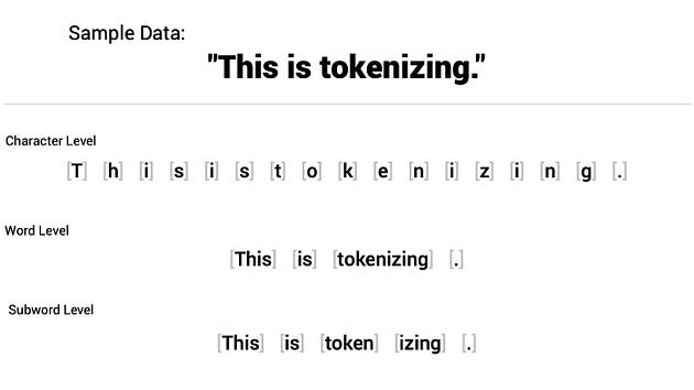
对句子进行分词后，我们根据分词器训练期间训练语料库中存在的创建词汇将每个分词映射到唯一的整数 ID。每个整数代表词汇表中的一个特定单词。

除了训练语料库中的单词外，Transformer 还使用特殊标记来实现特定目的。我们将立即定义以下一些内容：

• [UNK]：该标记用于识别序列中的未知单词。

• [PAD]：填充标记以确保批次中的所有序列具有相同的长度，因此我们用此标记填充较短的句子。我们使用注意力掩码“告诉”模型在训练期间忽略填充的标记，因为它们对任务没有任何实际意义。

• [SOS]：这是一个用于表示句子开始的标记。

• [EOS]：这是一个用于表示句子结束的标记。

在build_tokenizer下面的函数中，我们确保标记器已准备好训练模型。它检查是否存在现有的分词器，如果不存在，则训练新的分词器。

python">def build_tokenizer(config, ds, lang):
    tokenizer_path = Path(config['tokenizer_file'].format(lang))
    
    if not Path.exists(tokenizer_path): 
        
        tokenizer = Tokenizer(WordLevel(unk_token = '[UNK]')) # Initializing a new world-level tokenizer
        tokenizer.pre_tokenizer = Whitespace() # We will split the text into tokens based on whitespace

        trainer = WordLevelTrainer(special_tokens = ["[UNK]", "[PAD]", 
                                                     "[SOS]", "[EOS]"], min_frequency = 2) 
    
        tokenizer.train_from_iterator(get_all_sentences(ds, lang), trainer = trainer)
        tokenizer.save(str(tokenizer_path)) # Saving trained tokenizer to the file path specified at the beginning of the function
    else:
        tokenizer = Tokenizer.from_file(str(tokenizer_path)) # If the tokenizer already exist, we load it
    return tokenizer # Returns the loaded tokenizer or the trained tokenizer